Authoring Docs With Notebooks

Beautiful Technical Documentation with nbdoc and Docusarus

nbdoc is a lightweight version of nbdev that allows you to create rich, testable content with notebooks. Docusarus is a beautiful static site generator for code documentation and blogging. This project brings all of these together to give you a powerful documentation system.

Setup

1. Follow the Getting Started guide in the README to install and configure things appropriately.

2. Next, create an isolated python environment using your favorite tool such as conda, pipenv, poetry etc. Then, from the root of this repo run this command in the terminal:

   make install

3. Then you need to open 3 different terminal windows (I recommend using split panes), and run the following commands in three seperate windows:

   Note: we tried to use docker-compose but had trouble getting some things to run on Apple Silicon, so this will have to do for now.

   Start the docs server:

   make docs

   Watch for changes to notebooks:

   make watch

   Start Jupyter Lab:

   make nb

4. Open a browser window for this tutorial http://localhost:3000/docs/nb.

Authoring In Notebooks

For this tutorial to make the most sense, you should view this notebook and the rendered doc side-by-side. This page is called "Authoring Docs With Notebooks" This tutorial assumes you have some familiarity with static site generators, if you do not, please visit the Docusarus docs.

Create Pages With Notebooks

You can create a notebook in any directory. When you do this, an associated markdown file is automatically generated with the same name in the same location. For example intro.ipynb generates intro.md. For pages that are created with a notebook, you should always edit them in a notebook. The markdown that is generated can be useful for debugging, but should not be directly edited a warning message is present in auto-generated markdown files.

However, using notebooks in the first place is optional. You can create Markdown files as you normally would to create pages. We recommend using notebooks whenever possible, as you can embed arbitrary Markdown in notebooks, and also use raw cells for things like front matter or MDX components.

Front Matter & MDX

The first cell of your notebook should be a raw cell with the appropriate front-matter. For example, this notebook has the following front matter:

---
title: Authoring Docs With Notebooks
---

Consult the Docusaurus docs on front matter to see the various options available to you.

Markdown

You can include any markdown in markdown cells. One markdown feature that can be really useful for docs is for rendering diffs. A diff code block can be specified like this:

```diff
+ added this line
this line is the same
- deleted this line
```

And is rendered as like this:

+ added this line
this line is the same
- deleted this line

Static Site Generator Features

Since you can write markdown in notebooks, you can also take advantage of your static site generator's markdown features. For, example this site uses Docusarus, which means you can use any of its special markdown features such as admonitions or tabs.

Python Code

Code cells and output will show up in the docs as you would expect:

print('hello world')

hello world

Python Scripts In Docs

If you use the %%writefile magic, the magic command will get stripped from the cell, and the cell will be annotated with the appropriate filename as a title to denote that the cell block is referencing a script. Furthermore, any outputs are removed when you use this magic command.

This is what the cell input looks like:

%%writefile myscript.py

class MyClass:
    @classmethod
    def run(cls):
        return "hello world"

if __name__ == "__main__":
    print(MyClass.run())

The output is then rendered like this:

myscript.py

class MyClass:
    @classmethod
    def run(cls):
        return "hello world"

if __name__ == "__main__":
    print(MyClass.run())

Running shell commands

You can use the ! magic to run shell commands. When you do this, the cell is marked with the appropriate language automatically.

python myscript.py

hello world

It is often smart to run tests in your docs. To do this, simply add assert statements. These will get tested automatically when we run the test suite.

result = !python myscript.py
assert result == ["hello world"]

But what if you only want to show the cell input, but not the output. Perhaps the output is too long and not necesary. You can do this with the #meta:tag=hide_output comment:

print("".join(["This output would be really annoying if shown in the docs\n"] * 10))

You may want to just show the output and not the input. You can do that with the #meta:tag=hide_input comment:

You can only see the output, but not the code that created me
You can only see the output, but not the code that created me
You can only see the output, but not the code that created me

If you want to hide both the input and the output, you can use the #meta:tag=hide comment:

Running Tests

To test the notebooks, run make test. This will execute all notebooks in parallel and report an error if there are any errors found:

Skipping tests in cells

If you want to skip certain cells from running in tests because they take a really long time, you can place the comment #notest at the top of the cell. For example the below cell will not be tested. Go ahead, run make test from the root of the repo both with and without the #notest comment to see the different behavior.

assert 1 == 1

Formatting code with black

You can choose to format specific code cells with black with the comment #meta:tag=black, or manually adding the cell tag black in the Jupyter interface. For example, notice how the below code is reformatted in the rendered docs:

For example, this is the input code cell:

#meta:tag=black
j = [1,
     2,
     3
]

Becomes this:

j = [1, 2, 3]

This works with %%writefile as well.

For example, this input:

%%writefile black_test.py
#meta:tag=black

def very_important_function(template: str, *variables, file: os.PathLike, engine: str, header: bool = True, debug: bool = False):
    """Applies `variables` to the `template` and writes to `file`."""
    with open(file, 'w') as f:
        pass

Becomes this:

black_test.py

def very_important_function(
    template: str,
    *variables,
    file: os.PathLike,
    engine: str,
    header: bool = True,
    debug: bool = False
):
    """Applies `variables` to the `template` and writes to `file`."""
    with open(file, "w") as f:
        pass

DataFrames

Pandas Dataframes will be displayed per normal:

import pandas as pd
url = 'https://github.com/outerbounds/.data/raw/main/hospital_readmission.csv'
pd.read_csv(url).head().iloc[:, :3]

	time_in_hospital	num_lab_procedures	num_procedures
0	14	41	0
1	2	30	0
2	5	66	0
3	3	63	0
4	5	40	0

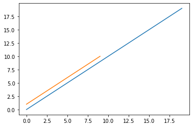
Plots

You can generate plots with many plotting libraries, which will automatically show up in the docs.

from matplotlib import pyplot as plt
plt.plot(range(20), range(20))
plt.plot(range(10), [x+1 for x in range(10)])
plt.show()

You can even have interactive charts with altair. Please note that all interactive plotting libraries may not work due to collisions between the static site generator and the plotting library. If you encounter issues, we suggest saving your plot as an image file to disk then displaying it with a markdown cell.

Interactive Plots

import altair as alt
from vega_datasets import data

source = data.cars()

alt.Chart(source).mark_circle(size=60).encode(
    x='Horsepower',
    y='Miles_per_Gallon',
    color='Origin',
    tooltip=['Name', 'Origin', 'Horsepower', 'Miles_per_Gallon']
)

caution

You should be careful when using interactive plots. Interactive pltos can inject lots of HTML into the page, which can slow things down significantly. Only create interactive charts when they are helpful.

You can instruct altair to render a chart as a static svg image with this line of code.

alt.renderers.enable('svg')

In order for this to work, you will have to install the altair_saver package.

Here is the same chart as a static image:

import altair as alt
from vega_datasets import data

source = data.cars()

alt.renderers.enable('svg')
alt.Chart(source).mark_circle(size=60).encode(
    x='Horsepower',
    y='Miles_per_Gallon',
    color='Origin',
    tooltip=['Name', 'Origin', 'Horsepower', 'Miles_per_Gallon']
)

Running Tests & Updating Notebooks

See this README section for more information on this topic.